The interaction between ocean waves and sea ice is a fundamental process that influences both the dynamics of the ice cover and the characteristics of the wave field.
Understanding how waves decay as they propagate through sea ice is crucial for improving our ability to model and predict ice-ocean interactions, particularly in the marginal ice zone (MIZ) where wave-ice interactions are most pronounced.
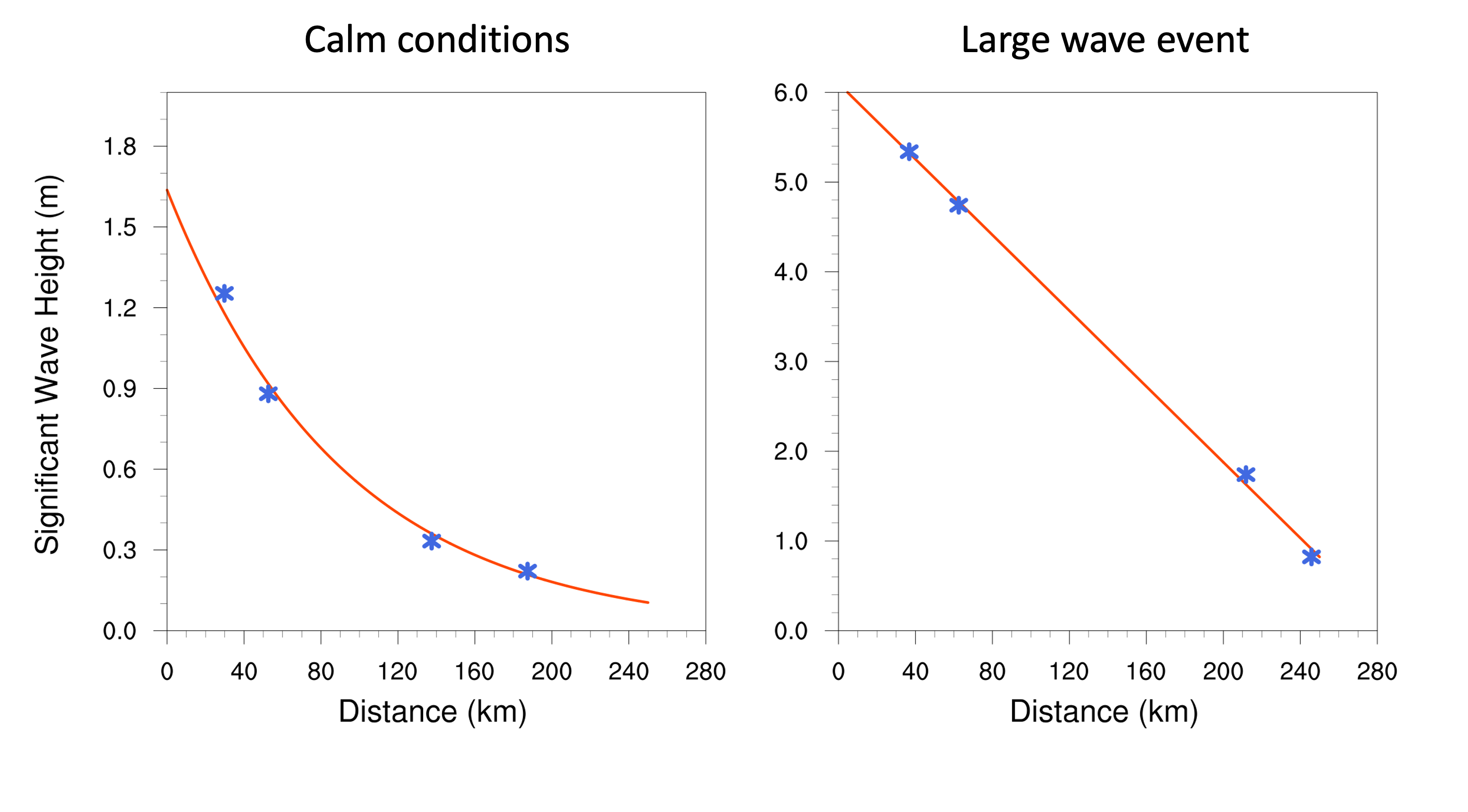
Figure 1: Wave decay in the marginal ice zone during a calm wave event and a large wave event. Each plot shows the significant wave heights as a function of distance from the ice edge from the WIIOS units (blue markers) and an exponential fit to the calm condition units and and linear fit to the large wave event (red line).
This understanding has become increasingly important as climate change leads to more frequent and intense wave events in polar regions, potentially accelerating ice break-up and affecting maritime operations.
Traditional approaches to studying wave decay in sea ice have relied on linear wave theory, but recent observations suggest this may not fully capture the complexity of wave-ice interactions, particularly during large wave events.
Analysis of wave decay in sea ice focuses on understanding the evolution of the full wave spectrum propagating through the ice.
Linear theory assumes that as a wave propagates through ice, the power at each wave number decays without transfer of energy between wave numbers.
This implies that the significant wave height, which is proportional to the square root of the total wave energy, will always decay exponentially with distance from the sea ice edge.
Our SIPEX data set confirms previous observations that, during calm conditions, the significant wave height decays exponentially with distance.
However, during three large wave events, we found that significant wave heights did not decay exponentially, enabling large waves to persist deep into the pack ice.
See Figure 1 for an example of these two cases.
To demonstrate the consistency of this, for our whole data record, we calculated the decay rate of the significant wave height between wave buoys, dHs/dx, where Hs is the significant wave height and x the distance between buoys.
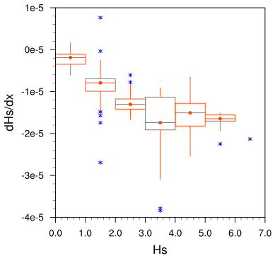
We present this data in the form of a boxplot (Figure 2), where we observe that the magnitude of dHs/dx increases almost perfectly linearly with Hs until Hs reaches 3 m, as we would expect for exponentially decaying waves as show in the calm plot in Figure 1.
Figure 2: Decay rates of waves for given significant wave heights.
Data are binned in 1-m boxes.
The red dot is the median.
Box height shows the range within which 50% of the data lie.
The whiskers give the range of data, excluding outliers (blue markers) and single data points (Kohout et al. 2014).
Code Snippet: Downsampling Implementation
/******************************************************************************
* Function: decimate
* Purpose: Decimates (downsamples) a signal after applying an anti-aliasing
* Butterworth filter
*
* Parameters:
* in[] - Input signal array
* out[] - Output decimated signal array
* sr1 - Input sampling rate (Hz)
* sr2 - Output sampling rate (Hz)
* n1 - Length of input array
* n2 - Length of output array
*
* Returns:
* void
*
* Notes:
* - Implements 2nd order Butterworth filter
* - Supports two specific sampling rate combinations:
* 1. 8 Hz input (sr1=0.125) with 0.5 Hz cutoff
* 2. 64 Hz input (sr1=0.015625) with 2 Hz cutoff
* - Requires integer ratio between input and output sampling rates
* - Includes bounds checking and error logging
*
* Filter Coefficients:
* 8 Hz sampling: a = [1.0, -1.4542, 0.5741]
* b = [0.0300, 0.0599, 0.0300]
* 64 Hz sampling: a = [1.0, -1.7238, 0.7575]
* b = [0.0084, 0.0169, 0.0084]
*
*****************************************************************************/voiddecimate(longdouble*in,longdouble*out,floatsr1,floatsr2,intn1,intn2){logger("Start decimate",0.0);inti,j,ii,n,jj;intstep;longdoubleout1[n1];longdoublea[3],b[3];logger(" n1",n1);// intialize outfor(i=0;i<n2;i++)out[i]=0.0;// butter worth filter with 8 Hz sample rate and 0.5 Hz cut offif(sr1==0.125){logger(" Butter worth filter with 8 Hz sample rate, 0.5 Hz cut off",0.0);a[0]=1.000000000000000;a[1]=-1.454243586251585;a[2]=0.574061915083955;b[0]=0.029954582208092;b[1]=0.059909164416185;b[2]=0.029954582208092;}// butter worth filter with 64 Hz sample rate and 2 Hz cut offif(sr1==0.015625){logger(" Butter worth filter with 64 Hz sample rate, 2 Hz cut off",0.0);a[0]=1.000000000000000;a[1]=-1.723776172762509;a[2]=0.757546944478829;b[0]=0.008442692929080;b[1]=0.016885385858160;b[2]=0.008442692929080;}if(!floorf(sr2/sr1==sr2/sr1)){debug("Error: step a non integer",0.0);return;}out1[0]=in[0];out1[1]=in[1];for(i=2;i<n1;i++){out1[i]=b[0]*in[i]+b[1]*in[i-1]+b[2]*in[i-2]-a[1]*out1[i-1]-a[2]*out1[i-2];}step=sr2/sr1;logger(" step",step);for(i=0,j=0;i<n1;i+=step,j++){if(j>=n2){fprintf(stderr,"ERROR: out of bounds in decimate. Exiting.\n");exit(0);}out[j]=out1[i];}logger("End decimate",0.0);return;}
For waves larger than 3 m, dHs/dx flattens and can be treated as being independent of Hs, as demonstrated in the large wave event plot in Figure 1.
This showed that existing linear theory appears to be only valid for waves with Hs < 3 m.
The empirical model derived from the data was
$$
\frac{dH_s}{dx} =
\begin{cases}
-5.35 \times 10^{-6}H_s, & H_s \le 3\,\mathrm{m} \\
-16.05 \times 10^{-6}, & H_s \ge 3\,\mathrm{m}
\end{cases}
$$
where $-5.35 \times 10^{-6}$ is the attenuation coefficient (Kohout et al. 2014).
The constant attenuation for waves with significant wave height greater than 3 m implies a more gradual decay of wave height with propagation distance, allowing large waves to penetrate considerably farther into the ice.
Because the ice in the MIZ was all first-year ice, we are unable to determine how equation (1) will differ in thicker ice or in a combination of first-year and multi-year ice.
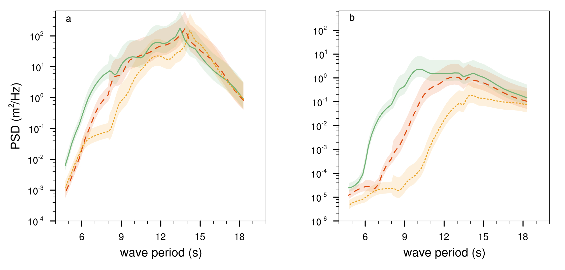
The wave spectra during large wave events indicate that the spectral peak of the energy distribution may shift to longer periods with increasing distance from the ice edge (Figure 3).
This is standard for waves in the open ocean, where nonlinear interactions create an inverse energy cascade, moving energy and the spectral peak to longer periods.
Figure 3:
The power spectral densities during a storm-generated wave event (a) and during calm seas (b).
For each event, the red dashed lines show the output of the unit closest to the ice edge and the yellow furthest from the ice edge.
The shaded regions give the 90% confidence intervals (Kohout et al. 2014).
Thus, our observations suggest that nonlinear energy transfer may need
to be considered when modelling the decay of large waves (Hs > 3 m) through sea ice and that small amplitude wave theory cannot simply be extrapolated to large amplitude waves.
To verify these findings we conducted a much larger experiment during PIPERS.
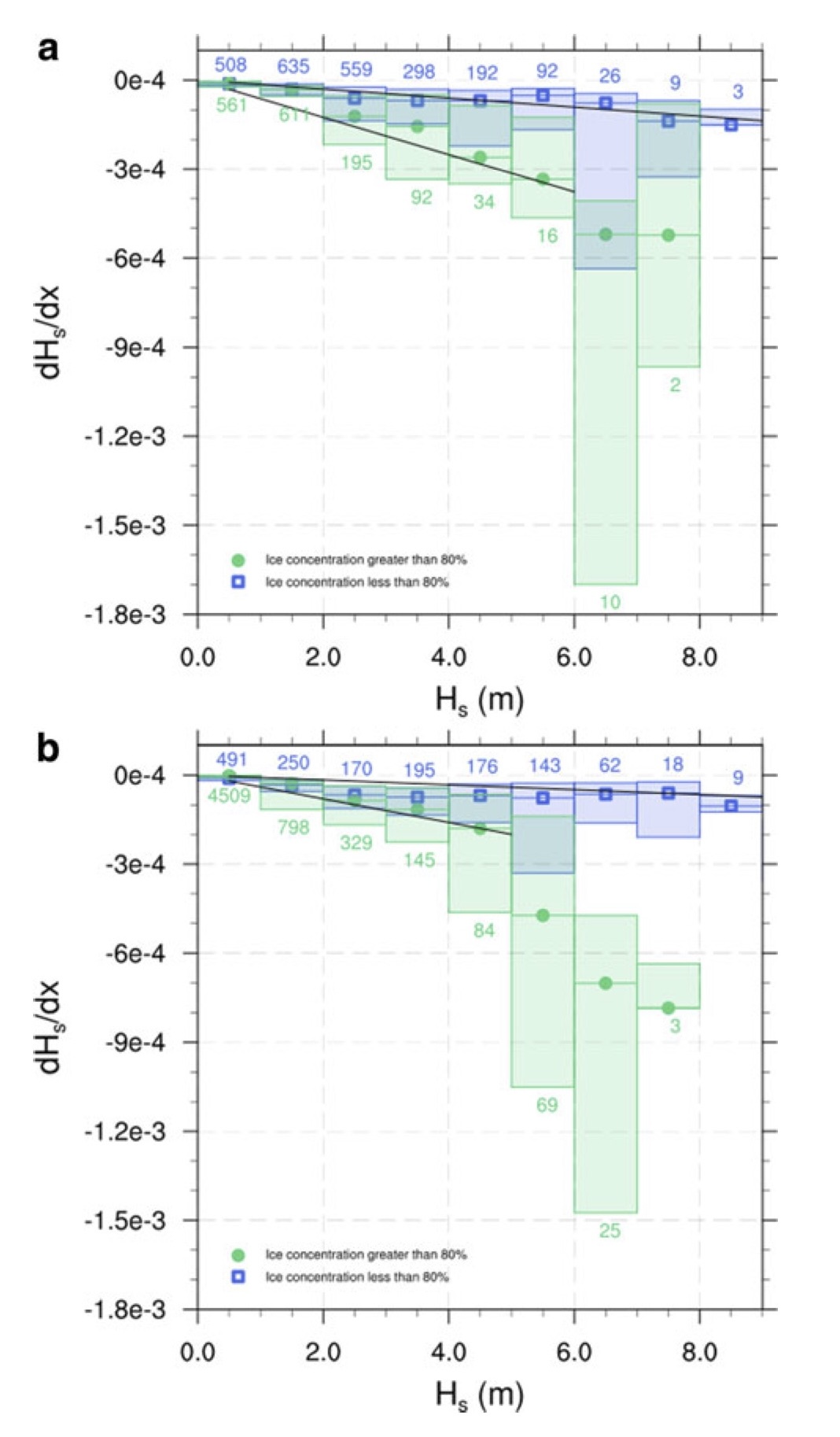
We again studied the decay rates and display the data in boxplots. This time however, the larger dataset allowed us to break the data into long and short peak wave periods and high and low ice concentrations (Figure 4).
This showed that generally during this experiment, the total wave energy decayed exponentially through the ice with the rate of decay dependent on ice concentration.
These results suggest that the conclusion from the SIPEX-II dataset, that large waves decay linearly, was likely an artefact of analysing a small dataset and comparing data experiencing differing ice conditions (Kohout et al. 2020).
Figure 4:
Decay rates of WIIOS in ice concentrations <80% (blue squares) and WIIOS in ice concentrations >80% (green circles).
(a) Data from WIIOS with peak periods <14 s.
(b) Data from WIIOS with peak periods >14 s.
Data are binned in 1 m boxes.
The markers are the median within each box.
The shaded boxes show the range within which 50% of the data lie.
The number of data points within each box is displayed above/below the box.
The black lines show the least-squares regression line of best fit to the median values within each box (Kohout et al. 2020).
For example, it is possible that during SIPEX-II, the large wave events predominantly occurred when low ice concentrations were present, thereby reducing the decay rates and leading to an appearance of linear wave decay.
Building on our experimental findings, we investigate the broader implications of wave breakup on sea ice extent.
We propose that increasing significant wave heights in the Southern Ocean enhance sea ice breakup, leading to a retreat of the sea-ice edge.
Conversely, decreasing wave heights would likely cause the ice edge to expand.
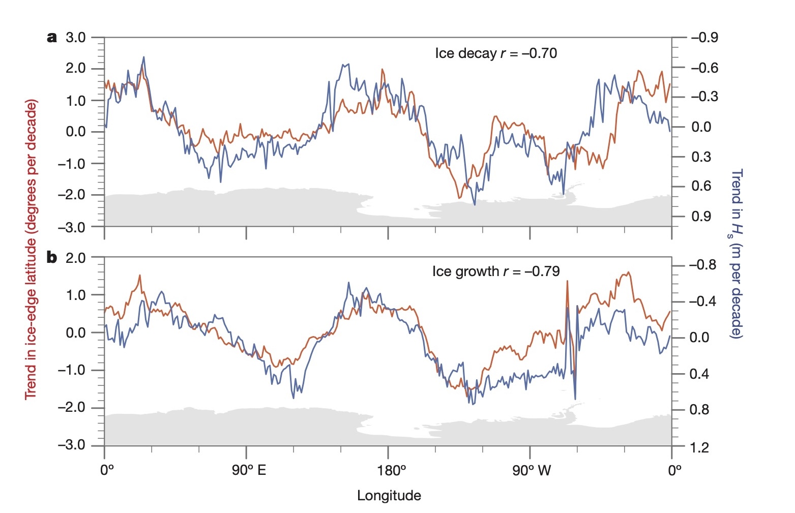
To test this relationship, we analyzed model-derived significant wave height estimates alongside satellite sea-ice observations from 1997-2009, defining the sea-ice edge at 15% ice concentration.
We divided the data into biannual seasons: growth (March-August) and decay (September-February) as shown in Figure 5.
Both seasonal analyses revealed that trends in sea-ice extent inversely correlate with significant wave height trends, with Pearson correlation coefficients of -0.70 during decay season and -0.79 during growth season (Kohout et al. 2014).
Figure 5:
A comparison between the trends in sea ice extent and significant wave height between 1997 and 2009.
The observed trend in the location of the ice edge (red) and the simulated trend in the significant wave height (blue) are shown as functions of longitude.
(a) Averaged trends for the ice decay season (September to February).
(b) The averaged trends during the ice growth season (March to August).
The Pearson coefficient (r) is given at the top right of each panel (n = 288 for each).
Antarctica is represented by the grey shaded region.
Note the scale for trend in Hs increases downwards (Kohout et al. 2014).
Our analysis indicates that a 2-meter increase in significant wave height over a decade corresponds to a 2° latitudinal retreat in ice extent (Figure 5).
Geographically, the most substantial wave height increases occurred in the Amundsen–Bellingshausen Sea, coinciding with documented sea-ice retreat, while the Western Ross Sea experienced the largest decreases in wave height, aligning with known ice expansion.
These 1997-2009 trends in wave height are consistent with observed longer-term patterns.
Our findings suggest sea ice vulnerability to changing storm patterns.
Recent decades have witnessed a southward shift in storm tracks, decreasing mid-latitude cyclones while increasing high-latitude cyclones.
This shift has not been uniformly zonal; recent trends in surface pressure and winds show zonally asymmetric changes, creating variability in atmospheric forcing on sea ice.
Future projections indicate increasing wave heights throughout Arctic and Antarctic sea-ice edges, potentially accelerating sea-ice retreat.